A little while back, there was a report from NYCDOT called Bus Forward. While I worked on some of the analysis in the report, one thing I noticed was that the analyst behind the maps included parks, despite them having little to do with bus speeds. Thanks to this report, I have started including parks in all of my map visualizations to help orient the intended audience. This technique only really works for local audiences, since folks with little knowledge of the city will not be able to use parks to orient themselves.

Finding the Data

Most open data websites for cities have shapefiles of parks that you can download. Chicago, Washington D.C. (National and Local), and Boston all have this information on their respective open data websites. If a city's open data website does not have the transit lines, you can typically find those in the developer area of an agency's site. Worst case you can try TransitFeeds, although sometimes the shapes.txt file there can be a little (or very) out of date.

Creating the Maps

For the Washington D.C. map, I used the shapefiles at the links below. Admittedly, D.C.'s geographic location makes this a little more complicated than it would be for other cities. However, once you have all of the shapefiles downloaded it becomes easy to add them to any visualizations you make.

• Metro Lines Regional
• Waterbodies
• Neighborhood Clusters
• National Parks
• Parks and Recreation Areas
• Maryland County Boundaries
• Virginia Cities and Counties

In order to import the shapefile into your QGIS project, simply drag the shapefile in. In the layers panel, rearrange the layers so the metro lines are on top, followed by waterbodies, national parks, and then parks and recreation areas. In the bottom right corner, change the projection (it is the button that says something similar to 'EPSG:4326') to NAD83(HARN)/Maryland (ftUS). This is EPSG:2893, the local projection that covers the D.C. area. This ensures Washington D.C. will look similar to how it looks on Google Maps and elsewhere.

To change the color of a layer, double click it, select symbology, select simple fill, and adjust the settings there. I used the following hex colors and settings for each layer:

• National Parks/Parks and Recreation Areas: #7caf83 fill color with 80% opacity, stroke style set to no pen
• Neighborhood Clusters and County Boundaries: #e0e0e0 fill color, #595959 stroke color
• Waterbodies: #a6cee3 fill color, stroke style set to no pen

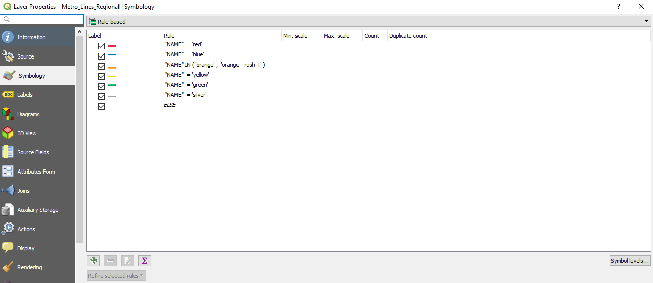
For the metro lines regional layer, switch the styling to rule based at the top of the symbology screen. I used the hex colors for each linea from here. To add rules, use the green plus button to add a rule. Click the epsilon symbol on the edit rule screen and enter in a script in the form "NAME"='color'. Do this for each line (with a slight change for the orange line), making sure your rules and colors look like the screenshot below.

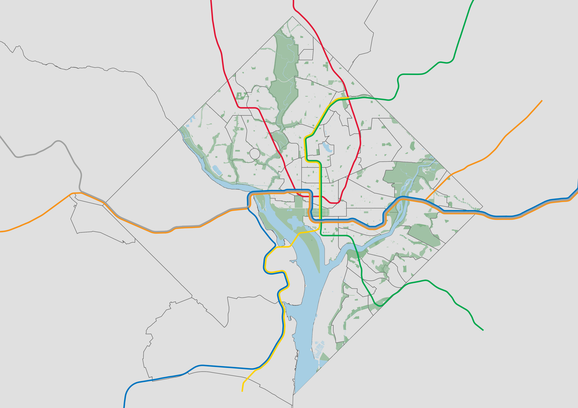
When you finish setting the colors, highlight all of the rules, right click, and change the width to 0.75mm. To make overlapping lines visible, I added an offset of -0.75mm to the blue line, 0.75mm to the orange line, and -0.75mm to the green line. The offset settings for lines are under the symbol section of the edit rule dialog. Click on 'Simple Line', and you should be able to find it. You may have to adjust these settings if you zoom in. If you did all of this, you should hopefully end up with map below!

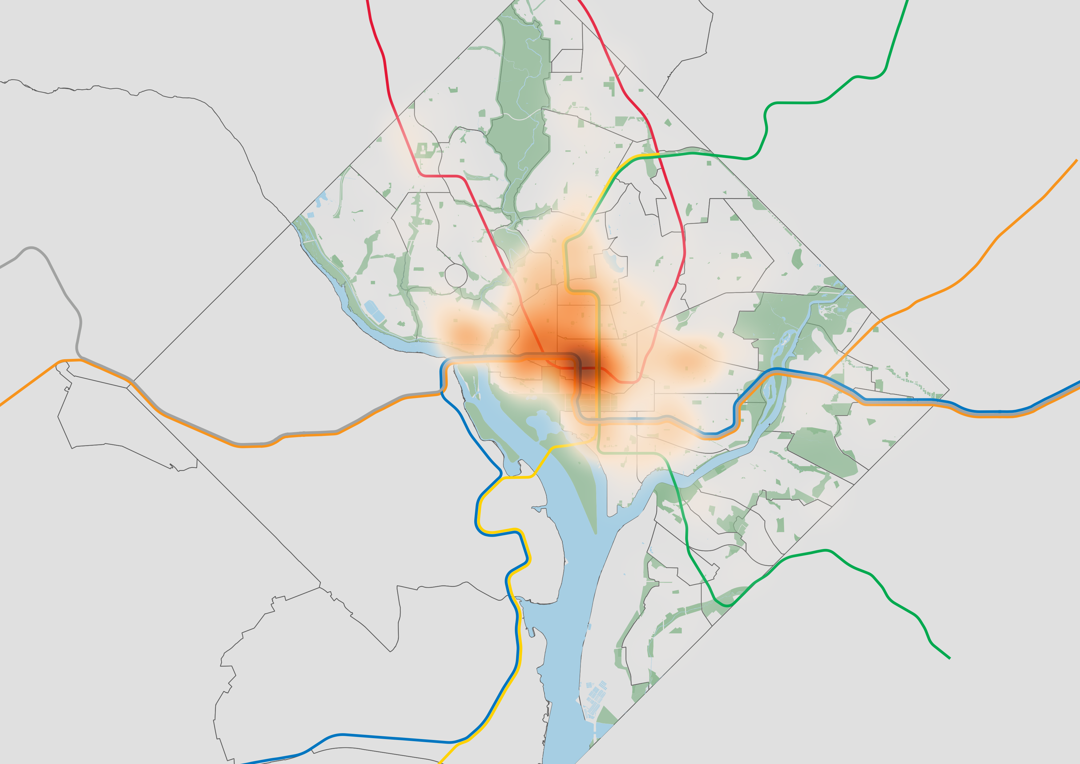
Final Thoughts

Looking at the base map above, most people familiar with the D.C. area should be able to identify geospatial patterns and how they affect different neighborhoods. However, this works better for some types of data than others. Data at the census block or neighborhood level will cover up all of these features. Personally, I have found heatmaps or line/point visualizations work best with this design. At different zoom levels, it may be useful to add metro stations, neighborhood name labels, and even individual streets. As a demonstration, here is an unsurprising heatmap of the 107067 parking violations in September 2017.