Using Checkers to Estimate Free Coffee Rates with Cluster Sampling

Taylor is in charge of Ockwell City's library system, and the city's leadership decided it wanted to promote reading by paying for a free coffee for every person in town who shows up at a coffee shop with the book they are reading. After much discussion, Taylor ended up in charge of measuring how many people actually brought in books to get their free coffee so that the city knows how much it will be on the hook for. While Taylor is not a statistician, they do have a leg up their sleeve. Their employee Tyne has designed samples before and knows just how to use their limited checker resources effectively.

Potential Alternatives to Statistical Sampling

While this is clearly a fantasy scenario, it is still worth addressing a few alternate methods that might work better in different situations than a statistical sample with checkers.

If you have a unified security camera database with high quality video, and behavior that is easy to identify with computer vision (e.g. crossing through ticket check at a movie theater), it would probably be better to develop a model that works off of the camera data you already have instead of sending checkers out. In this example though, different coffee shops likely use different security camera systems with varying levels of video quality and coverage.

If you have employees who can handle the additional cognitive load of recording the data directly, this will also provide a more reliable estimate than a statistical sample. In this case though, coffee shop employees may be too busy to record every single free coffee cup, or some more nefarious coffee shop owners may want to lie about how many free cups of coffee they gave out to get extra money from the city or appear more popular than they are.

One Stage Cluster Sampling

Our dutiful city employee Tyne knows we want to observe the proportion of coffee shop visitors who have books. The city only has one checker available for the measurement though, and Taylor has charged Tyne with estimating the citywide free coffee rate. He goes to the library and stumbles upon the diagram of different sampling methodologies below.

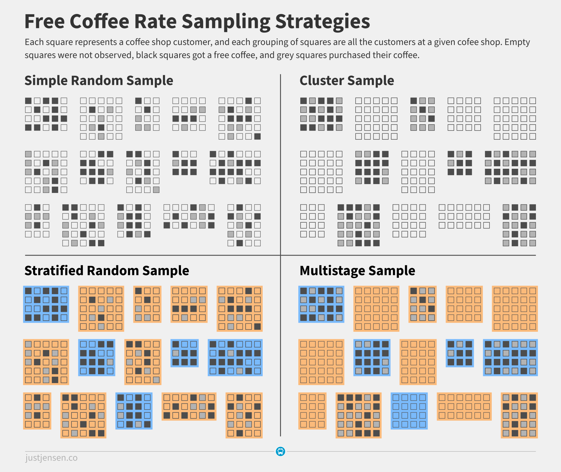
Unfortunately, this situation is not a simple random sample. In a simple random sample, Tyne's checker would be able to observe random coffee shop goers throughout the system. In this scenario though, the sampling unit is coffee shops, at which the checker will observe all elementary units, the coffee shop goers. This is known as a one stage cluster sample.

Tyne can pick coffee shops at random for the checker to observe, but can not pick which coffee shop goers walk into the coffee shop.

While a multistage sample (a stratified one-stage cluster sample) might be more efficient, the city has no prior knowledge about which types of coffee shops might draw book readers.

Sticking with the cluster sample approach, to get an equation for the free coffee rate estimate, we need to start by setting up some notation. Given the following:

$$\begin{align} n&=\mathrm{the\ number\ of\ clusters\ (coffee\ shops)}, \\ m_i&=\mathrm{the\ number\ of\ sampled\ persons\ in\ cluster}, \\ a_{ij}&=\mathrm{the\ smoking\ status\ of\ person\ }i\ \mathrm{in\ cluster\ }j  \end{align}$$

the free coffee rate is

$$r=\frac{\sum^n_{i=1} \sum_{j=1}^{m_i} a_{ij}}{\sum_{i=1}^n \sum_{j=1}^{m_i} m_{ij}}.$$

While there is a lot of fancy notation going on here, the above equation just means that to calculate the estimated free coffee rate, you need to sum up the total number of people who the checker saw using their book to get free coffee and divide that sum by the total number of coffee shop goers the checker observed. If the checker observed 15 entries, and 5 of them got their coffee for free, then the estimated free coffee rate would be \(\frac{5}{20}=25%\).

Developing a Confidence Interval Around the Free Coffee Rate

While the equation for the Free Coffee Rate is fairly easy to interpret and matches how you would calculate it in a simple random sample, defining the confidence interval is another story. Given \(\bar{m}=\), the average number of people the checker observes each check, then the variance \(v(r)\) is

$$\frac{\sum_{i=1}^n (a_i-rm_i)^2}{n(n-1)\bar{m}^2}.$$

The 95% confidence interval is then defined as

$$CI_{95\%}(r)=r \pm 1.96se(r)=r\pm 1.96\sqrt{v(p)}.$$

Walking Through an Example in R

Since we don't have access to the data that Tyne would have collected, we'll need to generate some in R. Let's assume that during the course of the program, the checker was able to visit 10 coffee shops. We will assume the free coffee rate is actually 25%.

# Start by generating a random number of observations for each of the ten
# coffee shops
set.seed(1)  # This way, your results match mine
num.observations <- floor(rnorm(10,mean=15,sd=5))
df <- data.frame(num.observations)

# The true free coffee rate, to compare to the estimate
true.free.rate <- .25

# Create a function to apply to the data frame to generate the number
# of evaders
f.sample <- function(x) {
  set.seed(1)
  return(sum(sample(0:1, x, replace=TRUE, prob=c(.75,.25))))
}
df$num.free.coffee <- apply(df, MARGIN=1, FUN=f.sample)

To get an idea of what the data looks like, see the dataframe we just generated below.

>df
   num.observations num.free.coffee ids
1                11               3   1
2                15               4   2
3                10               3   3
4                22               7   4
5                16               4   5
6                10               3   6
7                17               4   7
8                18               5   8
9                17               4   9
10               13               3  10

Now that we have a data set of surveys and observations, we can use the survey package to analyze it. We can now create a survey design object and generate an estimate of the free coffee rate along with a confidence interval.

library(survey)

df$ids <- as.numeric(rownames(df))
svy <- svydesign(ids=~ids, data=df)
svy.ratio <- svyratio(~num.free.coffee, ~num.observations, svy)
svy.confint <- confint(svy.ratio, level=0.95)

Now looking at the outputs,

> svy.ratio
Ratio estimator: svyratio.survey.design2(~num.free.coffee, ~num.observations, svy)
Ratios=
                num.observations
num.free.coffee        0.2684564
SEs=
                num.observations
num.free.coffee       0.01093617

>svy.confint
                                     2.5 %    97.5 %
num.free.coffee/num.observations 0.2470219 0.2898909

Given that the true rate is 25%, an estimate of 26.8% is not great, but not completely unreasonable either. Importantly, the true rate falls within our 95% confidence interval, and the interval is not too wide with an 8.0% margin of error relative to the free coffee rate estimate.

Addendum

Unfortunately for Tyne, not every example is as clear cut as an imaginary town where nobody lies about whether they are in fact reading a book to get a free coffee. Cluster sampling requires clusters to be similar in size to have an unbiased estimator. If one check is at Starbucks at 8:00 AM, while another check is at Bertha's Home-Roasted Beantown at 4:00 PM, this would likely violate that requirement. In addition, if there is heterogeneity between the clusters (the free coffee rate varies wildly between clusters) and homogeneity within the clusters, then the sample becomes less accurate.