The Department of Homeland Security (DHS) and the Office of the director of National Intelligence (DNI) issues a Joint Analysis Report (JAR) called GRIZZLY STEPPE. The analysis attributes the security compromises during the 2016 election to Russian actors who used Russian civilian and military infrastructure. While there is a good chance that Russian hackers attempted to influence the election, both Ars Technica and The Intercept have found the details of the public report lacking. It makes sense that security agencies would not give out all of their information to protect confidential sources, but this does not change the fact that almost half (49%) of the IP addresses in the Steppe Report are simply TOR Exit nodes.

Any state-sponsored (or independent) hackers should be able to do a reasonably good job of hiding their location, so the locations of these IP addresses probably will not help us glean much new information. Furthermore, GeoLocation is not always the most accurate way to identify location. Despite that, I have been meaning to learn QGIS, and I will likely need it for future projects at work. It's been 3 or 4 years since I last used ArcGIS for anything big, so it seemed like a good time to learn an open source alternative.

The Process

I downloaded the CSV file from US-CERT, processed the IP addresses to get them in a xxx.yyy.zz.nn format, and used the short R script below from Robert Grant's blog (his actual blog here). Notice that it requires the rjson package.

ip.addresses <- read.csv('IPAddressTor.csv', colClasses=c("character"))

freegeoip <- function(ip, format = ifelse(length(ip)==1,'list','dataframe'))
{
  if (1 == length(ip))
  {
    # a single IP address
    require(rjson)
    url <- paste(c("http://freegeoip.net/json/", ip), collapse='')
    ret <- fromJSON(readLines(url, warn=FALSE))
    if (format == 'dataframe')
      ret <- data.frame(t(unlist(ret)))
    return(ret)
  } else {
    ret <- data.frame()
    for (i in 1:length(ip))
    {
      r <- freegeoip(ip[i], format="dataframe")
      ret <- rbind(ret, r)
    }
    return(ret)
  }
}

locations.df <- freegeoip(ip.addresses$FBI_ADDRESS)
write.csv(locations.df, file = "IPAddressGeoLocated.csv", row.names = FALSE, na="")

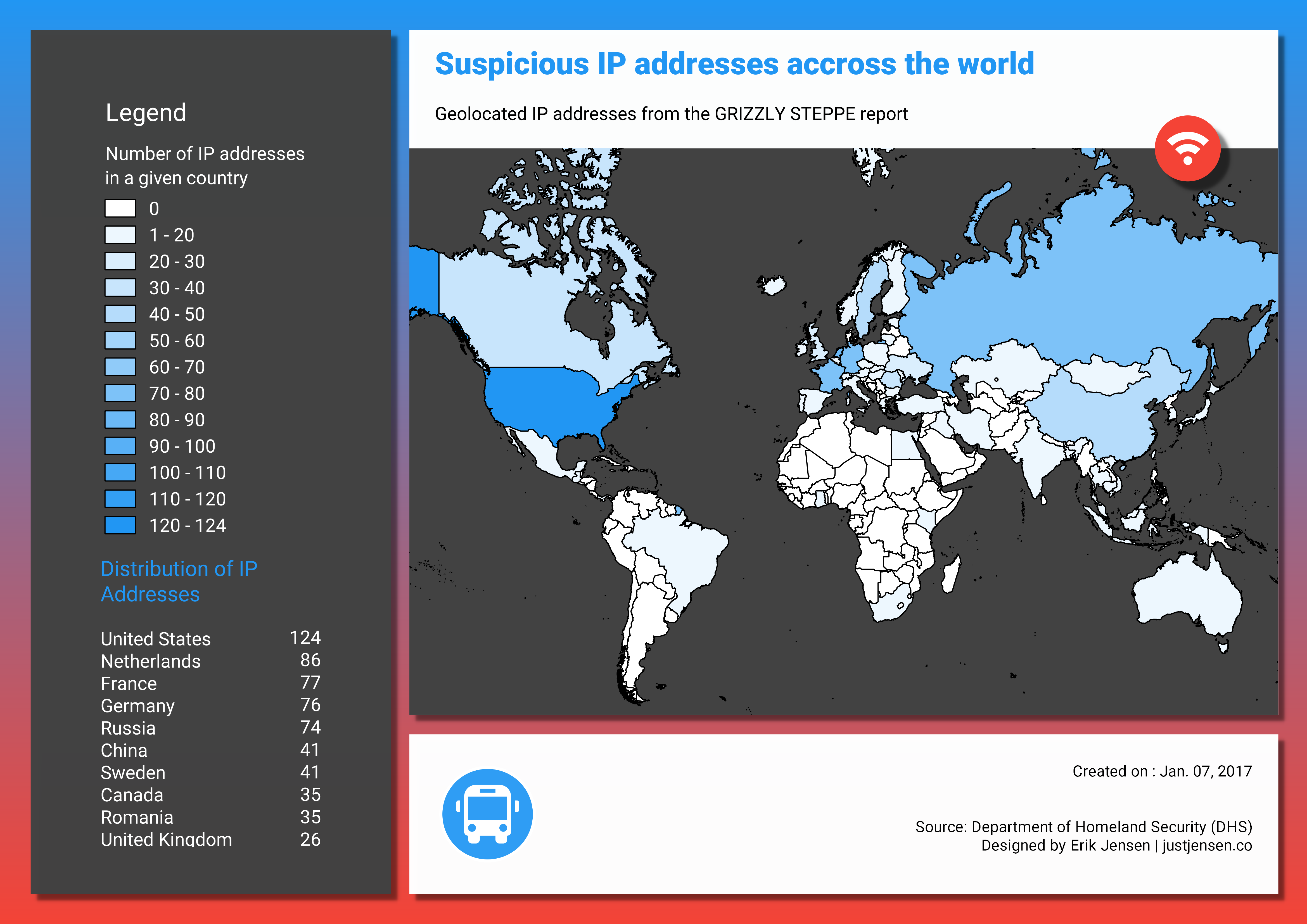
I then imported the output into QGIS as point data and used the country shapefiles from Natural Earth. I used the tool in Vector -> Analysis Tools -> Count Points in Polygon to count the number of IP addresses in each country. I followed the tutorial from Mickael HOARAU on Anita Graser's blog using my own choice of Material Design colors (they don't look quite as good). The output is below, and I think it turned out pretty well for my first map in 3 years. If I made it again, I would use the less detailed shapefiles from Natural Earth so there would be fewer islands showing up as black dots cluttering the map.